Big O Notation

Constant Time: O(1)

No matter how large the input, the algorithm will always take the same amount of time to complete.

Example: Accessing an element in an array by index.

def get_first(my_list):
    return my_list[0]

The function above will require only one execution step whether the above array contains 1, 100, or 1000 elements. As a result, the function is in constant time with time complexity O(1).

Linear Time: O(n)

Linear time is achieved when the running time of an algorithm increases linearly with the length of the input. This means that when a function runs for or iterates over an input size of n, it is said to have a time complexity of order O(n).

Example: Iterating through an array.

# Iterating through an array
def print_all_elements(my_list):
    for element in my_list:
        print(element)

The above function will take O(n) time (or "linear time") to complete, where n is the number of entries in the array. The function will print 10 times if the given array has 10 entries, and 100 times if the array has 100 entries.

Logarithm Time: O(log n)

When the size of the input data decreases in each step by a certain factor, an algorithm will have logarithmic time complexity. This means as the input size grows, the number of operations that need to be executed grows comparatively much slower.

To better understand log n, let's think of finding a word in a dictionary. If you want to find a word with the letter "p", you can go through every alphabet and try finding the word, which is linear time O(n). Another route you can take is to open the book to the exact center page. If the word on the center page comes before "p", you look for the word in the right half. Otherwise, you look in the left half. In this example, you are reducing your input size by half every time, so the number of operations you will need to perform significantly reduces compared to going through every letter. Thus you will have a time complexity of O(log(n)).

Example: Binary search and finding the largest/smallest element in a binary tree are both examples of algorithms having logarithmic time complexity.

def binarySearch(lst, x):
    low = 0
    high = len(lst)-1
    # Repeat until the pointers low and high meet each other
    while low <= high:

        mid = low + (high - low)//2

        if lst[mid] == x:
            return mid

        elif lst[mid] < x:
            low = mid + 1

        else:
            high = mid - 1

    return -1

The Binary Search method takes a sorted list of elements and searches through it for the element x. With every iteration, the size of our search list shrinks by half. Therefore traversing and finding an entry in the list takes O(log(n)) time.

Quadratic Time: O(n²)

The performance of a quadratic time complexity algorithm is directly related to the squared size of the input data collection.

Example: 2 nested for loops.

# 2 nested for loops
def print_all_possible_ordered_pairs(my_list):
    for first_item in my_list: # O(n)
        for second_item in my_list: # O(n)
            print(first_item, second_item)

We have two nested loops in the example above. If the array has n items, the outer loop will execute n times, and the inner loop will execute n times for each iteration of the outer loop, resulting in n² prints. If the size of the array is 10, then the loop runs 10x10 times. So the function will print 100 times. As a result, this function will take O(n²) time to complete.

Exponential Time: O(2ⁿ)

With each addition to the input (n), the growth rate doubles, and the algorithm iterates across all subsets of the input elements. When an input unit is increased by one, the number of operations executed is doubled.

# Iterating through all subsets of a set
def print_all_subsets(my_set):
    all_subsets = [[]]
    for element in my_set:
        for subset in all_subsets:
            all_subsets = all_subsets + [list(subset) + [element]]
    return all_subsets

# or

def naive_fibonacci(n):
    if n <= 1:
        return n
    return naive_fibonacci(n - 1) + naive_fibonacci(n - 2)

In the above example, we use recursion to calculate the Fibonacci sequence. The algorithm O(2ⁿ) specifies a growth rate that doubles every time the input data set is added. An O(2ⁿ) function's exponential growth curve starts shallow and then rises rapidly.

O(n!) — Factorial Time Complexity

describes algorithms whose running time grows factorially with the input size n

Factorial growth is extremely steep, making these algorithms infeasible for large inputs. Even for relatively small n (e.g., n = 10), the number of operations can become overwhelming (10! = 3,628,800).

Factorial time typically arises in problems that require generating all possible permutations or combinations with constraints.

# Iterating through all permutations of a set
def generate_permutations(arr, start=0):
    if start == len(arr) - 1:
        print(arr)
    for i in range(start, len(arr)):
        arr[start], arr[i] = arr[i], arr[start]
        # Recurse
        generate_permutations(arr, start + 1)
        arr[start], arr[i] = arr[i], arr[start]

O(1): Constant space.

The algorithm uses a fixed, unchanging amount of memory, regardless of input size.

This means no additional memory is allocated that grows with the input.

def print_all_elements(my_list):
    for element in my_list:
        print(element)

Why O(1)? Even though we're iterating over the list, we're not creating any new data structures that grow with the list. The only extra space used is for the loop variable element, which is reused on each iteration.

O(n): Linear space.

The algorithm uses linear amount of memory, proportional to the input size.

The memory used grows linearly with the input size. If the input doubles, the space used also doubles.

Example: Iterating through an array and storing the values in a hash table.

# O(n) space - Storing all elements in a hash table
def reverse_list(arr):
    reversed_arr = []
    for i in range(len(arr) - 1, -1, -1):
        reversed_arr.append(arr[i])
    return reversed_arr

Why O(n)? We create a new list reversed_arr that holds all elements of the original list in reverse order. This new list has the same size as the input, so the space required grows proportionally to n.

O(n²): Quadratic space.

The memory used grows proportionally to the square of the input size. If the input doubles, space may quadruple.

Example: Iterating through an array and storing the values in a 2D array.

# O(n²) space - Storing all elements in a 2D array
def create_identity_matrix(n):
    identity = [[0 for _ in range(n)] for _ in range(n)]
    for i in range(n):
        identity[i][i] = 1
    return identity

Why O(n²)? We're creating an n x n 2D matrix (a list of n lists, each with n elements). The total number of stored elements is n * n, leading to quadratic space usage.

O(2ⁿ): Exponential space.

The memory used doubles with each additional input element. For n items, there are 2ⁿ possible subsets, so space grows very fast.

Example: Iterating through all subsets of a set.

# Exponential Space - O(2ⁿ)
def power_set(arr):
    result = [[]]
    for item in arr:
        result += [subset + [item] for subset in result]
    return result

Why O(2ⁿ)? For a set of size n, the powerset has 2ⁿ subsets. Each of these subsets is stored in the result list, leading to exponential growth in memory usage as n increases.

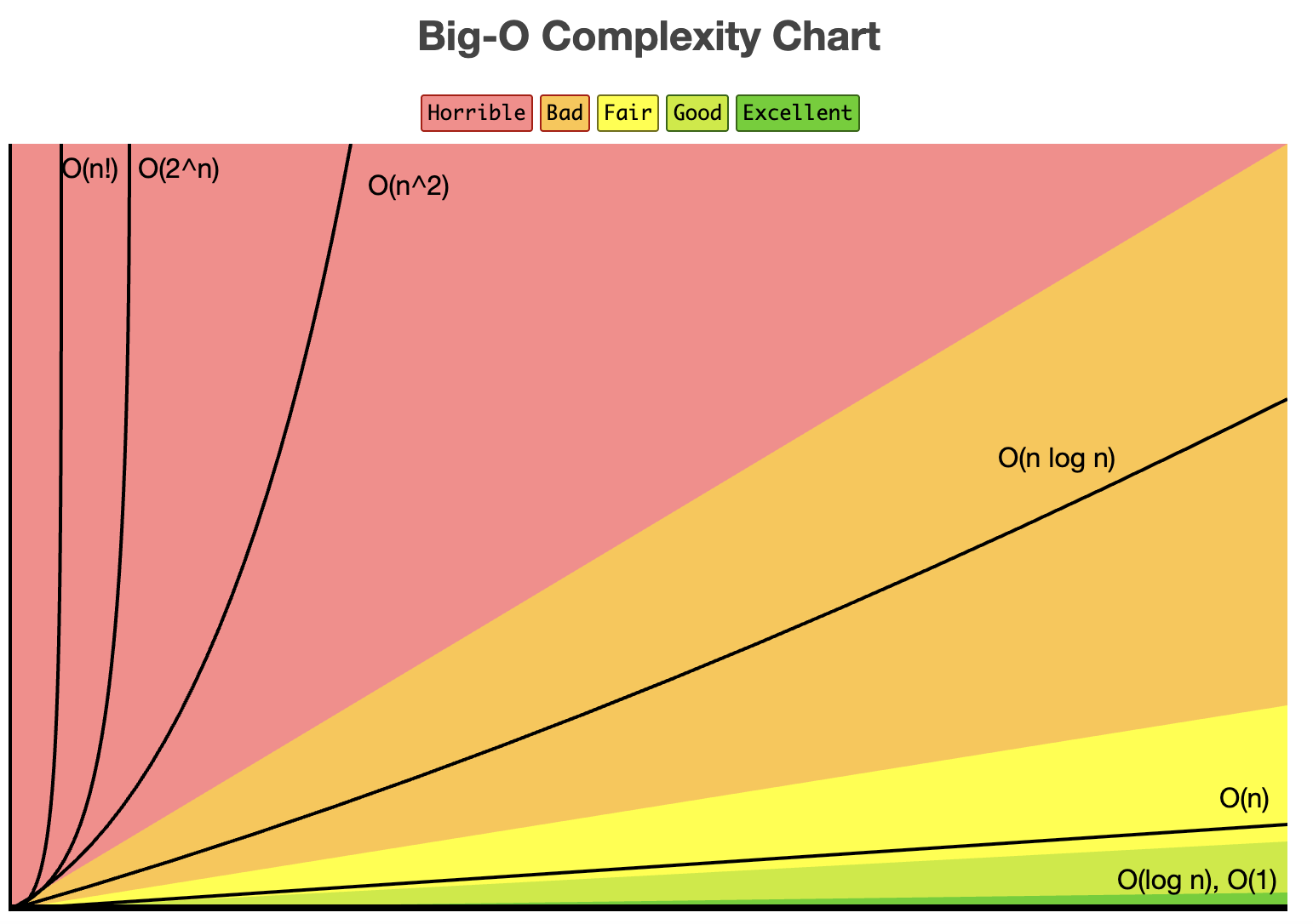
Big O Notation Complexity Chart